An Important Test for the Global Growth Cycle
Whatever kind of strategy you're employing as an investor, an invaluable tool for determining it's usefulness is testing. Not simply backtesting on historical data or stress testing on synthetic data – that's the easy part. The fun and playful part. A much more important test comes with a strategy's performance on new, real-time data.
A couple of months have passed since I've published the Global Growth Cycle strategy. Today, a first test of the methodology in real time is possible – due to a fresh sell signal occurring after the latest monthly data for November 2021.[1]
You can read more on the details on the strategy in the growth article, but in short it can be summed up as follows: the strategy relies on publicly available OECD economic data, published monthly. A Diffusion Index of OECD Composite Leading Indicators for each of the provided countries is calculated,[2] and a crossing of 50% up is considered a buy signal (global growth entering an expansion phase), a crossing of 50% down is considered a sell signal (growth entering a contraction phase). That is the Global Growth Cycle (GGC) model. In the GGC strategy I've added a simple market timing procedure (employing a moving average), whenever the model signals a contraction.
The most recent signal as of first publishing the strategy has been a change from contraction to expansion phase after the data for May 2020. Thus far the strategy has only been a backtest. In the following months new data have been published, and we can now check on the strategy in real time. The newest release (data regarding Nov 2021, released on Dec 9, 2021) suggests growth switching – from expansion to contraction – after 20 out of 39 countries have had a contracting CLI print month over month. Less than 50% are growing. In other words: a sell signal.
A very important caveat of this data, and the methodology in general, is that – as all economic data – it is subject to revisions. Especially now, when the number of contracting countries' CLIs outnumbers the growing countries solely by one – the signal is frail and is subject to revisions. But due to the averaging nature of the Diffusion Index, one might hope, the revisions should not have an important impact over a longer term. The signal might turn out to appear a month earlier or two months later than today, after a future data revision, but it should not turn out to be, for example, a year later.
Let's take a closer look at the current economic cycle relative to previous ones. Figure 1 shows the current standing of the diffusion index relative to all other paths after a "contraction phase ending" signal (the recent one being May 2020). 2009, 2016 and 2020 paths pre- and post-signal are highlighted.
Hover over years above chart to see specific cycle signals highlighted.
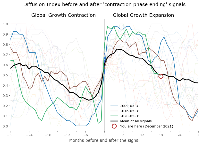
If we assume the data not to "revise the signal out of existence" in the near future, the current expansion phase appears to be coming to an end. It would be a bit shorter than the 2009 and 2016 expansions – by about 3 to 6 months. The recent expansion would last 1.5 years. The time between the previous switch from expansion to contraction (Feb 2018) would be 45 months – in line with historical precedents, considering the historical mean cycle period of 2.67 years (for the origin of these number see the typical expansion section of the growth article).
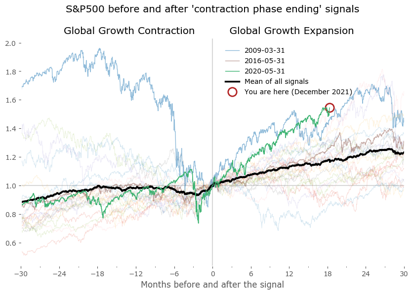
The performance of the S&P500 index meanwhile, has been one of the best for any expansion phases of the strategy, as of 18 months later, see Figure 2. It's been relatively stable on the way up, not experiencing any severe downturns (like the post-2009 expansion had in 2010, for example). If the signal turns out to be false (and revised data will show no down-crossing of the 50% line of the Diffusion Index), what history suggests is a continuation of uptrend, as visualized by the mean of all signals, shown here as a wide, black line.
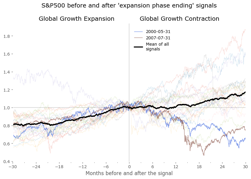
If, on the other hand, we get a confirmation of the recent signal, switching the current environment from expansion to contraction, Figure 3 highlights what can be further expected. These are S&P500 paths after all "expansion phase ending" signals. Not all resulted in "bearish" markets, but some did (such as the 2000 and 2007 cases highlighted) and the mean of all signals suggested a flat, tougher road ahead for stocks for the next 12 to 16 months (black widened line). In other words, a contraction phase, after which the next expansion phase typically follows.
Assuming perfect future information...
We will have to wait for future data to determine the duration of the current expansion cycle and if indeed the sell signal is correct, but meanwhile I've come up with a useful visualization of the buy and sell signals, and why I think the recent sell signal might be important.
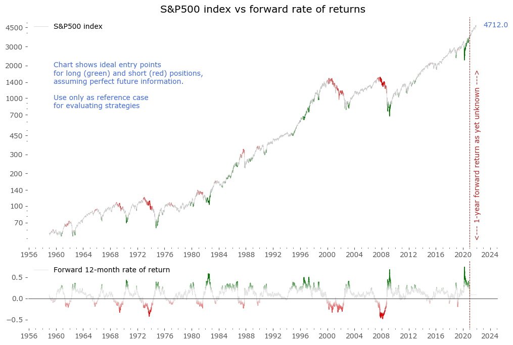
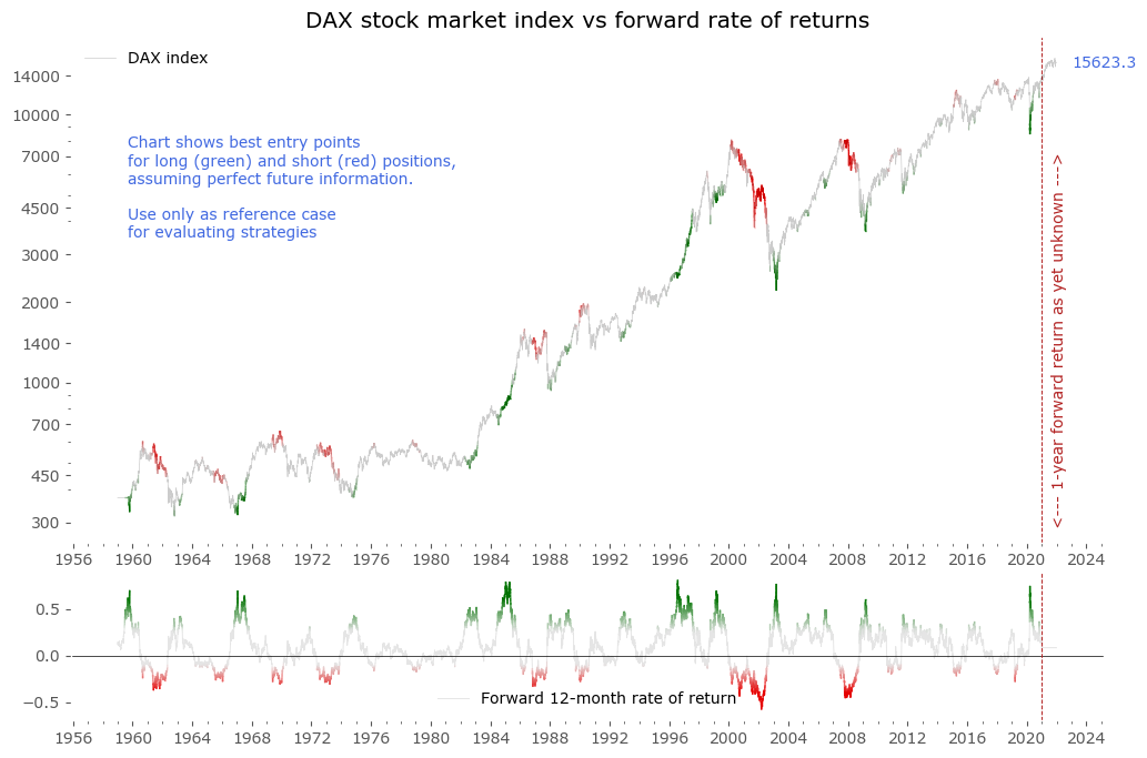
Let's have a look at the best and worst times to buy or sell a market index. One way to this is to look at some longer term rates of return of the index. Figure 4 below shows 12-month returns, but with a twist: the returns are shifted backwards in time, and are then used as a color palette for the main stock market index. That way we obtain a chart showing the absolute best and worst times to be long the stock market index, assuming a 1-year horizon and a perfect knowledge of the future.
Two such experiments are presented: for the S&P500, and for the DAX index.
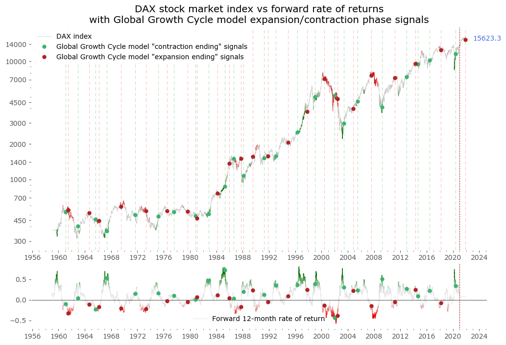
Let's now overlay this chart with all the OECD CLI's Diffusion Index expansion / contraction phase change signals – pictured in Figure 5. There are quite a lot of them, so the chart has become pretty crowded – I've included them as datapoints (green / red), and as dashed vertical lines in the exact dates. I've also plotted them on the forward returns below the chart.
What is clearly visible is that some of them timed the market perfectly, while others where not so lucky. What is convenient, the "unlucky" signals have been usually reversed in a couple months' time – replaced by a consecutive reverse phase signal. What is most important, and crucial for the model to be of practical use, is that the average of all "buy" signals (green) is above 0 on the forward rate of return – the higher, the better for the success of the model. And the average of the "sell" signals (red) is below 0. Which is a nice graphic representation, that a year forward has been (on average, although it might be very different for specific signals) successful for both of these signal types – the green ones usually preceded one-year future gains, the red ones usually preceded one-year future losses.
Ideally we would like to see a predictive model sell during the red areas of the "perfect information" color-coded index and buy during the green areas. That is: exit in an environment that will turn out to be harder for stocks, and enter in an environment that will turn out to be favorable. While certainly not perfect, we see that the GGC methodology does quite a good job – it usually enters the market (a green signal) after the turn of market index from a price low, but not too much higher. The exits (red signal) are more erratic – sometimes before, sometimes after a recent price high, but generally not bad also.
Discussion
Looking in to the specifics, one of the worst buy signals (lowest green points on the forward rate) occurred in 1965 – and was reversed 6 months later. Also unsuccessful was the signal from 2001 – reversed 5 months later. Among the worst sell signals (highest red points on the forward rate) is the one in 1989, after which the market index rallied somewhere near +30%, before reversing all this price appreciation a year later; and in 1997, after which a similar rally occurred, yet the model switched back to expansion more than a year later.
Most other signals were quite successful, especially the buy signals in 1967, 1989, 1993, 1996, 2003, 2009, 2016 and after the covid-crash of 2020. Noteworthy are also the good exit signals of the 1960s, 1987 (a large bit of luck there, I suppose, just 2 months before the crash), 2000, 2007, 2011 and 2018.
With the recent deterioration of CLI growth among OECD countries, a fresh Global Growth Cycle model "expansion ending" signal appears to be generated. Will it prove to be as much a successful signal as the best ones listed above? Or will it quickly be reversed into a "new expansion starting" phase? And most importantly – will it be confirmed or turn out premature and the revised data published in a few months will show no signal at all? Whatever the outcome, the current environment will be the first important real-time, live test of the model and, consequently, the Global Growth Cycle strategy. Even if the revisions invalidate the signal, meaning the current expansion phase will turn out to be longer, the "end of expansion" signal will have to trigger eventually. And how the market behaves after that, should be a good indication if the model stands the test of out-of-sample market data, and how strongly OECD data revisions weigh on the model's predictive strength.[3][4]
Due to the longterm uptrending nature of equity markets, the currently ongoing test can be of greater value: after all, it's a lot easier to predict a further uptrend in a market that is uptrending most of the time. A correct (or, at least, close) timing of a price high in such an environment is a lot harder and would be more convincing of the usefulness of a market timing strategy. Smart and very intelligent people have tried and failed at predicting a downturn during the current very strong bull market. A correct indication (either now, or sometime in the near future) of an end to this economic expansion would make the GGC much more interesting in my view (or at the very least, extremely lucky).
I've used the DAX index for comparing with the GGC signals, but that's not very important. Applying them to the S&P500 would result in similar conclusions. Of course, the specific CAGR and drawdown values of the model / strategy will vary (both are quantified in the growth article, see Table 2 of that article for specifics), but due to the correlated nature of market indices (especially during times of distress and downturns), the results will be largely similar. Some specific signals might be better or worse, but the overall picture does not vary significantly.