Extended Analysis of the GGCE Strategy
An extension of previous research on the Global Growth Cycle Enhanced strategy
Table of contents: Whipsaws in the GGCE, Drivers of the strategy's performance, Allocation Edge, Selection Edge, Returns by year, Summary and Discussion, References
5 years have passed since the original Global Growth Cycle was formulated[1], and 1 year since its simple modification, the Global Growth Cycle Enhanced[2]. The first important test of the methodology came at the end of 2021[3], with the first risk-off signal in real-time data, which successfully identified the risk of a bear market that materialized in 2022.
Since then, a risk-on signal in 2023 signaled a return to a risk-on environment and, apart from a brief risk-off episode later that year, remained in that state until the second half of 2026, which was also the right call.
A risk-off signal in July 2026 proved incorrect: the system switched back to risk-on in September, only to return to risk-off again this month, in November 2026.
Such signal filckering is nothing new or abnormal in trend-following strategies (as we will see later in the analysis), but it has prompted me to write a detailed analysis of the strengths and weaknesses of the approach, as well as to visualize similar episodes in the historical data available. I also want to take a closer look at allocation and selection edges, and show when each of these has made an important contribution to the overall result.
———As a side note: I've launched a new blog, in Polish, inwestowanieAlgorytmiczne.pl, focused on automation, algorithmic and systematic investing, but with a more casual, daily approach to trading and investing. It's been running for over a year now. Sometimes I discuss recent market events, sometimes I write in detail about specific strategies. The blog is aimed at a Polish audience (friends, family, coworkers and people interested in the subject), and most parts of this analysis have already been featured there.[4]
I imagine that, for most of you, the language barrier might be an issue. However, with today's LLM and AI capabilities, automatically translating the articles shouldn't be a problem. I encourage you to check it out.
If the current site, as I've written in the about section, is a library, the new blog is more of a curated forum – a public space where algorithmic investment topics can be discussed easily and more frequently. You're more than welcome to comment or contact me if you like. And to join the discussions.
I write without using AI, but I rely heavily on LLMs when writing code. I'm a big fan of the technology, and I believe that in the future, the original language of research and blogs won't be a real barrier, as translations will be pretty much seamless and automatic.
———Whipsaws in the GGCE
Whipsaws are a common feature of trend-following trading strategies. A great piece on such strategies, from both a theoretical perspective and a practical one, was written by Jesse Livermore (pseudonym) of Philosophical Economics in his (rather massive) article on the Growth Trend Timing strategy.[5]
The article starts with an extensive discussion of how trend following works, explaining whipsaws and gaps in such systems. The author explains very clearly the inevitable trade-off of having a closer match to the price trends we intend to capture (shorter MA-periods with quicker reaction times), but with more frequent whipsaws in return. The opposite is also true: longer MA-periods for measuring the trends are associated with fewer whipsaws, but also bigger gaps and later reaction times. I encourage you to read the article in full to understand and be fully aware of how such trend-following systems work, and why gaps and whipsaws are an inevitable, if painful, property of such systems.
Let's now focus on such whipsaws in the GGC strategy – episodes of frequent regime changes: from risk-on to risk-off and vice versa.
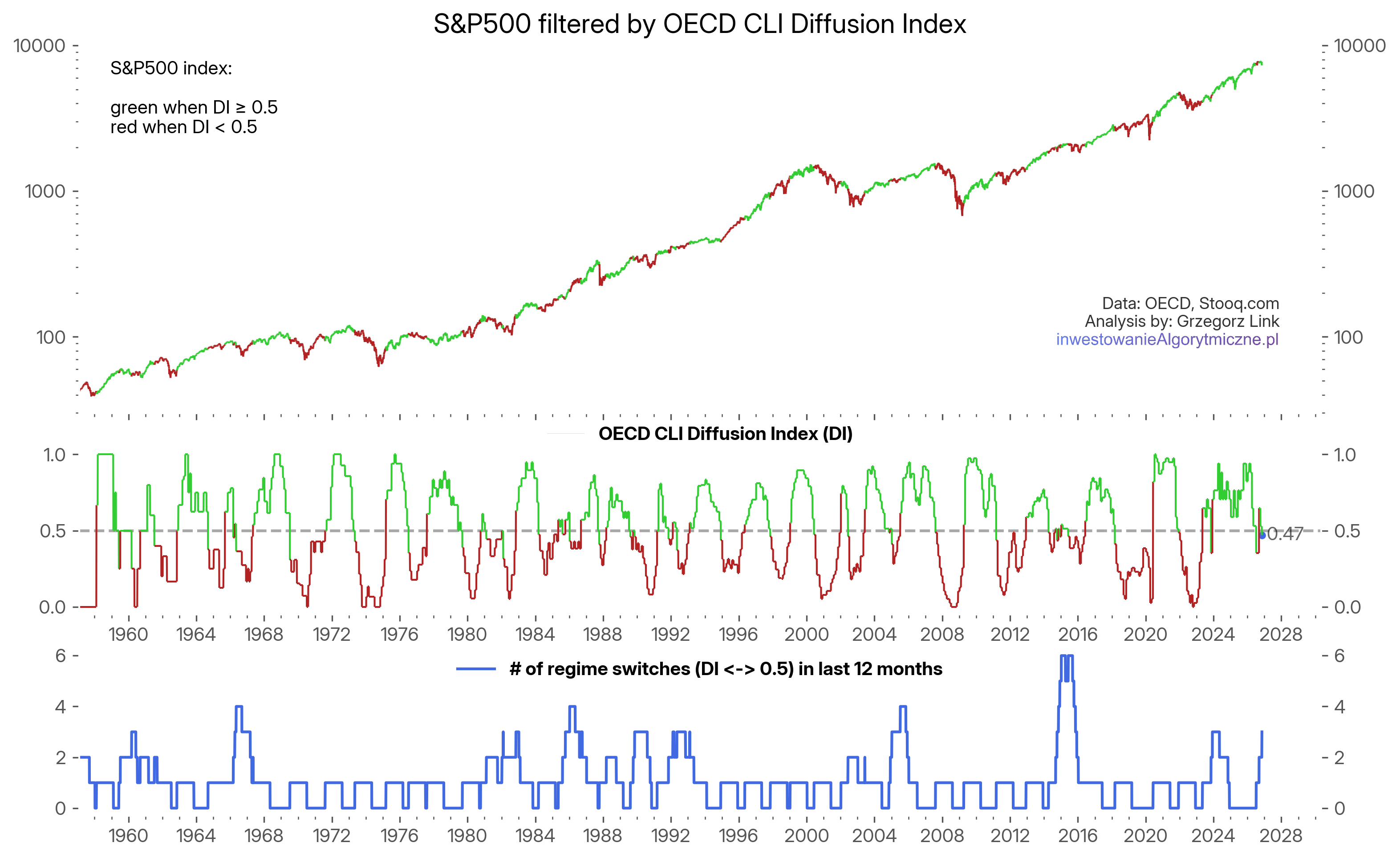
Figure 1 shows the full OECD Diffusion index data (in the middle panel), as well as the S&P500 index (upper panel) colored by the corresponding regions: green when at or above 0.5, and red when below. The cyclical nature of the Diffusion Index is clearly visible (though the cycles vary in length). The recent flickering activity, as well as the latest value of 47%, are seen near the end of the chart.
The lower panel of the chart shows the number of regime switches in the last 12 months. As you can see, the current value of 3 is no extreme: the highest values recorded have risen to as much as 6 switches in a year. Let's focus on those regions.
There have been 4 distinct events when the number of regime switches in a year has reached at least 4. In Figure 2, I've zoomed in on all four of those cases. All subcharts show a period of 3 years: 18 months before and 18 months after the moment they reached the maximum number of switches. The maximum number of switches was 4 in 1966, 1986 and 2005, and 6 in 2015.
The case in 1966 eventually helped avoid a strong bear market, but the system re-entered the market higher than exited before. Neither 1986 nor 2005 was followed by a meaningful bear market after switching to risk-off, and after a brief loss, both re-entered risk-on regimes eventually. The 2015 case is a bit similar to the 1966 one, as a (not especially large) bear market was avoided, though after 6 regime switches, 3 of which resulted in losses cumulatively similar in size as the bear market drawdown itself.
What is evident from these charts is that none of them is a clear winner in the task of providing returns higher than the underlying index, although two of them were successful in avoiding large drawdowns.
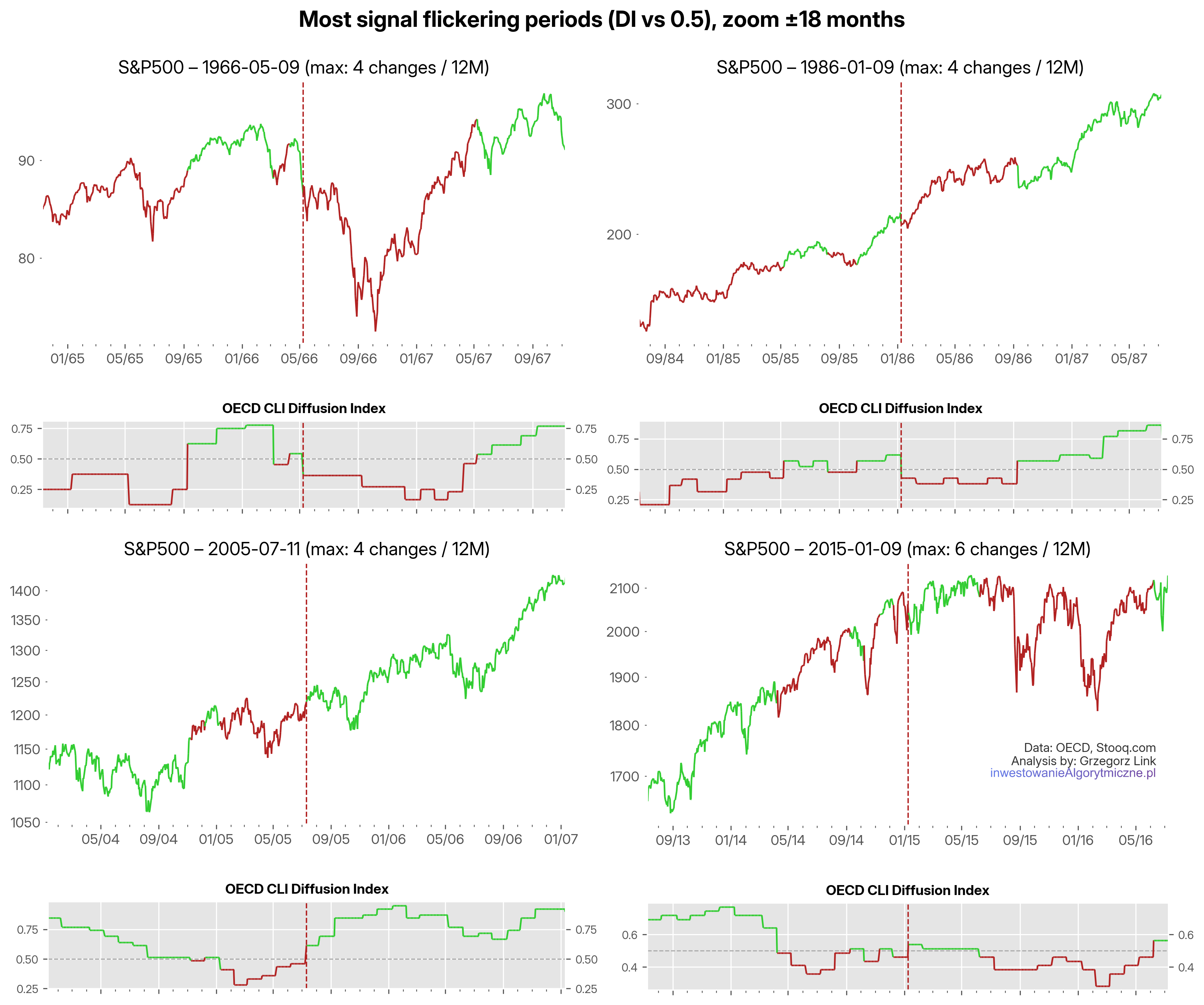
The main point is that the current episode of 3 signal flickerings is nothing extreme (yet), as even 6 switches during one 12-month period have occurred. And the only theoretical limit is 12 switches a year.
If such flickering is an annoyance, why should we stay in this strategy at all? What do we get in return for weathering all these storms and sticking to the signals in the long term? And what is the effectiveness of all these risk-on/off signals in the long term?
In other words – what is the strategy's advantage, what's the edge?
Drivers of the strategy's performance
To take a shot at the answer, let's look at an updated version of the total return from last year's article with latest data. Figure 3 shows the GGCE equity line in blue, S&P500 in orange. The data is from 1970 until today, covering 56 years, of which only 5 are out-of-sample (realtime data collected since I published the GGC strategy in 2021), the rest is just a backtest. Data for the ETFs are simulated (from corresponding indices) for the years before their inception.
The CAGR of the full strategy (15.9%) is over 4% higher than that of the index (11.3%), with the maximum drawdown substantially lower (-17.0% vs -50.7%). Those are the attributes we're aiming for.
I've added a green dashed line, named "Allocation only". This is simply the S&P500 during the risk-on only episodes (and BIL/IEF otherwise). In other words: what would be the result of only the allocation part of the strategy rules, disregarding the selection (SPY vs VXUS) rule. The CAGR of such a model (13.9%) sits somewhere between the pure index and the full GGCE, which gives us a crude estimation of how much return attribution comes from the allocation (risk-on/off) rule. Interestingly, it has a smaller maximum drawdown than the full strategy.
On the second subchart I've plotted total excess: the blue GGCE equity line divided by the buy&hold returns and normalized. What results is an estimate of the total excess return over the passive index.
By constructing the same measure for the allocation-only (green) equity line over buy&hold (orange), we arrive at the third subchart: an estimate of the total Allocation excess return. Similarly, comparing the GGCE equity line over the allocation-only line we arrive at the Selection excess return on the last subchart.
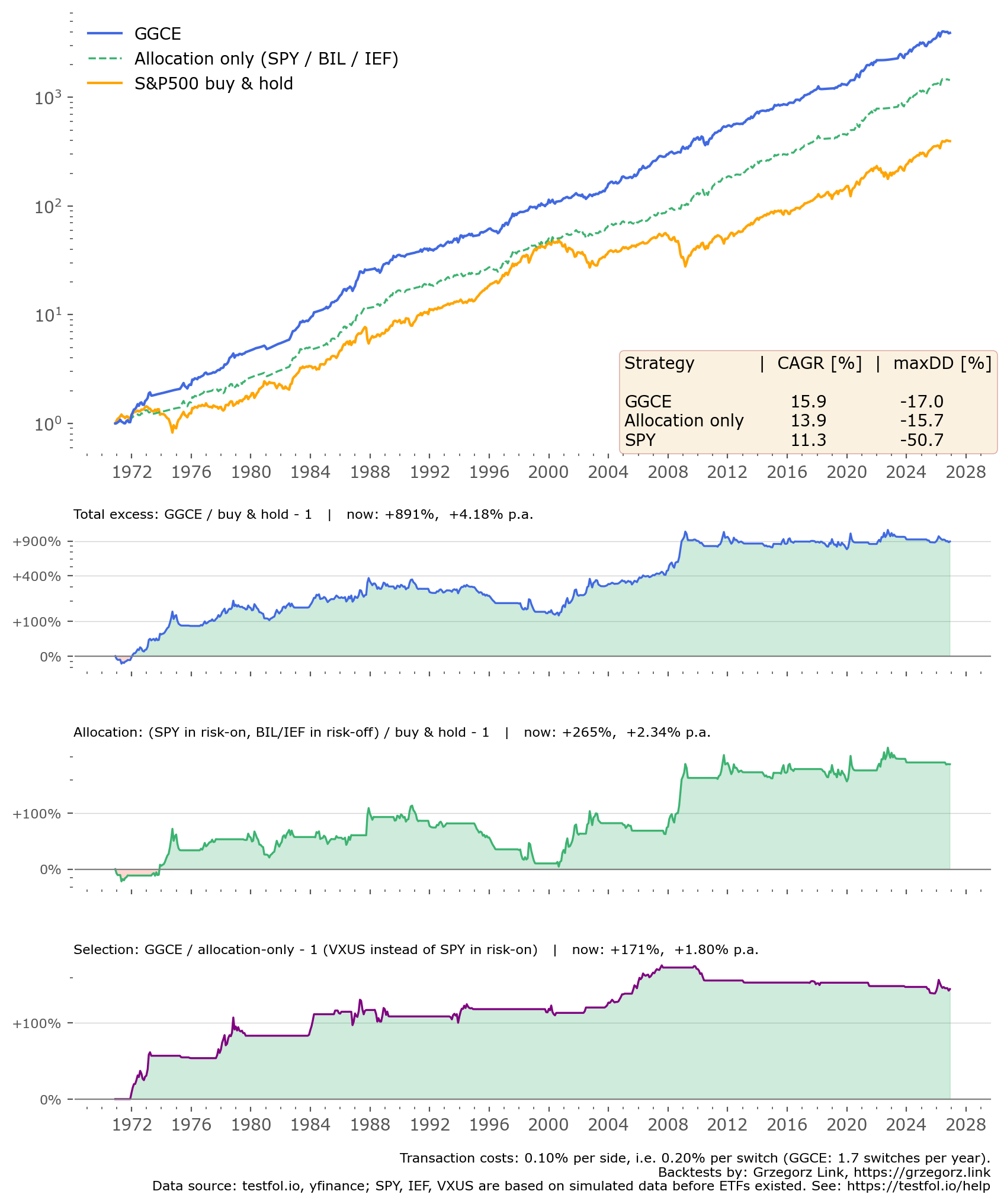
What is visible at first from the blue equity line is a clean, mostly smooth uptrend. But in reality, zooming in on some of these episodes reveals a lot going on, as we've seen in the previous zooms for whipsaw periods. It was not as easy to survive these episodes, as might seem from the equity line.
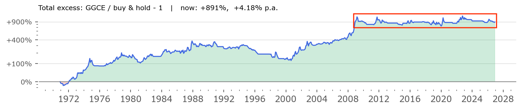
Figure 4 shows the same Total excess chart as in the second panel above, but I've highlighted a recent episode of activity with a red rectangle. We can see that through the ups and downs of the last ~17 years, this excess return is mostly flat. Which can be surprising – sticking with this strategy gives us mostly the same return as the buy&hold. So where's the edge?
The 4%+ overperformance over the passive index comes mostly from the earlier years: first a clearly rising trend from 1970s to the end of the 1980s, then a slightly falling trend, and a resurgence of overperformance from 2001 to 2009. There have been times when the strategy was still advantageous since 2009 (for example in the 2022 bear market) but the general excess is mostly flat.
Allocation Edge
To be clear, that isn't a bad outcome. Being inline with the market index, that has certainly one of the strongest returns in recent decades as the S&P500 has (see for example typical stock market returns in this study), while retaining much smaller drawdowns is still a big win. But it's important to understand where the edge of a strategy lies and what are the conditions needed for it to truly outperform.
In search of this understanding, let's zoom in on the Allocation and Selection parts of the excess return of GGCE. The 4.2% excess return is composed of:
- around 2.3% of outperformance due to allocation (correctly identifying risk-on and risk-off regimes),
- with the remaining 1.8% coming from the selection of US vs ex-US equities.
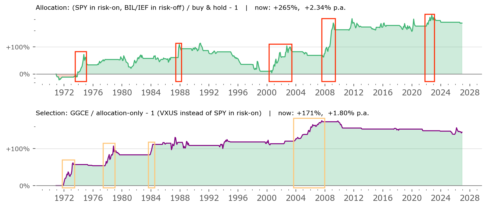
Figure 5 shows how that difference is distributed through time. On the upper subchart – allocation – I've plotted red rectangles showing periodical bursts of outperformance. The periods are: 1974, 1987, 2000-03, 2008 and 2022. An informed investor might easily identify those periods as simply the largest bear markets of the S&P500.
In other words: the allocation edge of the strategy comes mainly from avoiding exposure during most of the strong drawdown periods of the broad market. Avoiding bear markets. There were 5 such times in the last 56 years of data for the strategy. The rest of the time the allocation is mainly just chugging along, with even a period of severe underperformance during the strong technological bull market of the late 1990s.
Selection Edge
The lower subchart of Figure 5 shows the Selection excess returns. I've highlighted rising trends in orange – there are just 4 such periods, 1972-73, 1977-79, 1984 and 2003-07. Those are some of the periods when ex-US stocks performed clearly better than the S&P500 (but not all, as some outperformance periods happen outside of risk-on periods, when the strategy is allocated to cash or bonds).
What is worth noting is that the last such excess selection return period occurred over 19 years ago. That's a long time ago. The later period was mostly flat or even slightly falling. That means in practical terms it might be hard to convince today's investors of this specific selection mechanism, as for the last 19 years they wouldn't see any difference. If no difference, why bother?
The answer to that question is what I consider the strongest case for any such systematic strategy mechanism: we use it not to predict future outcomes, but to be prepared for them. We don't know when a bear market will develop, setting the stage for an allocation outperformance of the strategy. But if one does, these charts show clearly that the GGCE strategy should help us cope. We don't know when US stocks will fall out of favor, and the general investment community will drive more funds toward international equities. The last such episode was the 2003-07 bull market, during which US equities suffered relative underperformance. But if such a phenomenon happens again, we will be prepared.
Returns by year
Lastly, let's take a deeper look at the yearly returns and the specific contributions from each (allocation and selection) mechanism. In the table below, GGCE and SPY returns are shown. Alloc. only comes from the green, dashed equity line from Figure 3. From these numbers, we arrive at:
- the Excess: total excess (GGCE return over the SPY return).
- the Allocation contribution (Alloc. only return over the SPY return).
- the Selection contribution (GGCE return over Alloc. only return).
Keep in mind the returns are calculated as ratios, not differences. So for example (1 + Excess) = (1 + Allocation) × (1 + Selection).
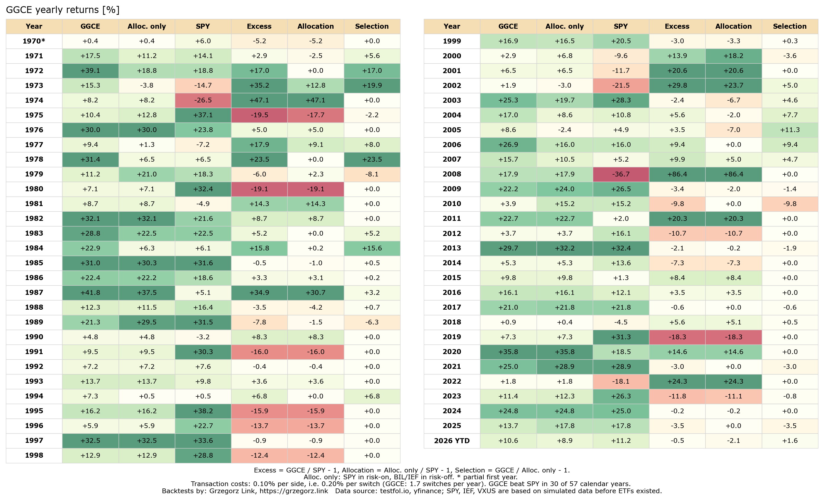
We see here in detail, what we already hinted at in the equity line charts: Selection worked best in 1972-73, 1978, 1984, and the 2003-07 period (most green periods for this column). Allocation delivered highest outperformance in years, when SPY had subpar returns, mainly bear market environments.
One can also see the strategy lagged the index mostly (most red in Excess column) during the 1995-99 period, as well as years just after a strong bear market: 1975, 1991, 2019, to a smaller degree 2023. It also lagged during the S&P500's strong year of 1980. Interestingly, the bull markets after the deepest bear periods (2000-03 and 2007-08) went quite well for the GGCE.
Summary and Discussion
The following segment is a translation of the same section in my Polish blog post on the subject.
This is a very simple strategy. You invest in ETFs and make decisions regarding asset allocation and selection once a month – that is, a maximum of 12 times a year, and often much less. Over a 56-year period, you would have made, on average, slightly fewer than 2 allocation adjustments per year (specifically, 1.7).
Simple but not easy. You have to carry out these adjustments at times that, in the short term, are often far from optimal. You must contend with the noise of information and resist the pressure to chase the returns you see generated by other strategies or sources around you. During the most powerful dot-com bull market (1995-1999), your performance would have lagged behind the broader market.
There will be false signals along the way. Whipsaws are the cost and inevitable feature of trend-following mechanisms. There were periods – as illustrated in Figure 1 – where you might have made as many as 6 allocation adjustments in a single year; the most recent instance was in 2015. 3 adjustments seen recently aren't extraordinary – the reality could be much more painful. If you intend to stick with this strategy, you must be prepared for the long haul.
However, the true strength and advantage of this approach become especially apparent during difficult periods – times of significant market turbulence or prolonged downturns.
The entire allocation edge proved beneficial only 5 times over the full 56-year span (all during bear markets), while the selection advantage came into play just 4 times (during periods when the U.S. market significantly underperformed the rest of the world). These few instances resulted in a compound annual growth rate (CAGR) that was 4% higher than the index, achieved with significantly smaller drawdowns than those experienced in passive investing.
Given this, is it worth drawing sweeping conclusions from these few isolated cases, or attempting to "fine-tune" the strategy to perfectly match current market conditions? I think it’s worth a try, but it’s important to remember that the strength of this strategy lies in its simplicity – whatever you decide to add to it, make sure you don’t compromise that simplicity.
This strategy certainly requires an extraordinary amount of patience and a good deal of faith: given that, over the last 19 years, there hasn’t been a single instance where the selection rule (switching to VXUS over SPY) has been advantageous, it will be difficult to convince many people of the need for such a mechanism. And since the strategy has already cycled three times in the last few months – without yielding results – some may find it hard to stick with it through another six or nine such cycles.
In my view, the primary source of the strategy’s edge is a behavioral play. Most investors will either choose not to adopt it or will drop out along the way, simply because it demands a very strong conviction. I happen to possess that conviction, but not everyone will – and I certainly wouldn’t recommend this strategy to someone who, for instance, prefers shorter-term investing, market timing, or chasing the latest bull run. For me, however, it is a suitable approach.
With tactical allocation you don’t need to predict the future.[6][7] You don’t have to guess when a bear market will arrive, nor whether the next bull market will be driven more by U.S. assets or otherwise. Instead, you trade the difficulty of making such predictions for the challenge of sticking with simple signals – signals that occur rarely but carry significant long-term weight.[8][9] In the short term, however, following them can be quite painful – relative to the rest of the market – over periods spanning months or even years.[10]
In essence, there is a behavioral trade-off: you don’t need to track vast amounts of information, you don’t need to guess, and you don’t need to predict. But you do need to have staying power and remain consistent.
Please keep in mind that the GGC strategy, with its risk-on/off regime switching, has been tested on real-life, out-of-sample data only for the past five years. Will it stand the test of time over the next 10, 20, or 30 years? Time will tell. I intend to continue sharing it publicly, along with its performance results. If you have ideas on how to improve it or adapt it for your own use, please feel free to do so – and do let me know. Every strategy should be tailored specifically to your own capabilities, risk preference and personal goals.